GOINT 001 : An introduction to Synthetic Aperture Radar (SAR) imagery.

This article serves as an introduction to SAR (Synthetic Aperture Radar) for GEOINT (Geospatial Intelligence) and OSINT (Open-Source Intelligence) applications.

This article serves as an introduction to SAR (Synthetic Aperture Radar) for GEOINT (Geospatial Intelligence) and OSINT (Open-Source Intelligence) applications. It is the first entry in a multi-part series aimed at introducing basic tools and knowledge to work with freely available satellite imagery for intelligence and monitoring purposes. We'll cover basic SAR principles and some preprocessing steps needed for further analysis.

This is not meant to be an exhaustive SAR course as certain aspects (like polarimetry, speckle, imaging modes) are intentionally left out, since they are not essential for the GEOINT/OSINT applications we’ll explore later.

8-bit vs 16-bit images :

Before diving into actual SAR image processing and interpretation, it's worth touching on some basic concepts related to how remote sensing data is stored and visualized. One of these is bit depth, which defines how many brightness levels each pixel can represent :

• 8 bits : Each pixel can have 256 possible values (from 0 to 255).

• 16 bits : Each pixel can have 65,536 possible values (from 0 to 65,535), allowing for a much finer distinctions in brightness levels.

Most consumer grade computer monitors are limited to 8-bit RGB for a total 16 Mil colors, meaning when displaying a 16-bit image on these monitor it will either be :

1. Compressed : A linear or nonlinear stretch is applied to map the original 16-bit pixel values into the 8-bit display range (0–255) with (0) : the minimum pixel value in the image and (255) maximum pixel value.
   Subtle differences between 2 images might not be visible.

2. Clipped or Truncated : Only a portion of the full data range is displayed, this can enhance contrast within that specific range, but the rest of the image's dynamic range is lost.

It is therefore important to apply appropriate histogram stretching and contrast adjustment when working with 16-bit data in order to properly visualize and interpret the image content.

Introduction to SAR remote sensing :

SAR (Synthetic Aperture Radar) is an active sensors that can either be mounted on satellite, UAV or an aircraft.
The active part means the sensor generates its own microwave signal and does not rely on sunlight. This guarantees imaging capabilities day or night, and even under cloud cover.

The radar emits microwave pulses toward the Earth's surface and listens for the echoes that return. For each resolution cell on the ground, the radar will pick up a signal comprised of the sum of all backscattered waves by objects within that cell. For an object to contribute to the received signal its radar cross-section (and not it's size) needs to be greater than the background noise of the radar.

This will give us 2 images :

1. Phase Image : Represents the average phase of the signal for each pixels. These images are not directly interpretable by humans and are used in pairs for interferometry (more on that on another article where we'll be talking about CCD)

2. Amplitude (or intensity) image : Represents the strength (intensity) of the backscattered signal. Intensity is equal to the amplitude squared which can displayed with either a linear scale or decibels (dB). This backscatter intensity depends on several factors; mainly surface roughness, moisture content, geometry of the target relative to the radar, and dielectric properties of the materials of the target. Higher pixel values indicate stronger backscatter, such as from urban areas, metallic objects or a slope facing the radar. On this article we'll focus on these images.

After radiometric calibration, the pixel values in an intensity image represent the radar backscatter coefficient, a physically meaningful quantity independent from sensor-specific effects (gain, antenna pattern...etc) ensuring pixel from different images or sensors are comparable.
This coefficient being either beta nought (β⁰), sigma nought (σ⁰) or gamma nought (γ⁰) the difference between them is the reference backscatter area used.

• Beta nought (β⁰) uses the slant range plane.

• Sigma nought (σ⁰) uses the CRS' ellipsoid taking into account the the incidence angle.

• Gamma nought (γ⁰) uses the topography and the the local incidence angle, after Radiometric Terrain Flattening.

Figure 1 : Reference backscatter area for Sigma, Beta, and Gamma Nought. (Gumelar O. et al., 2017).

We distinguish three main types of backscatter in SAR imagery, based on how the radar signal interacts with different surfaces and structures :

• Specular backscatter : where the radar signal reflects away from the sensor with little to no returns towards it which lead to these areas appearing dark/black on the image. Happens over calm water and smooth flat surfaces.

• Volumetric backscatter : where the signal penetrates into a medium like vegetation or snow and scatters in multiple directions, producing moderate returns.

• Double-bounce scattering : happens when the signal first hits a horizontal surface (like the ground), then reflects off a vertical structure (like a building wall) and back to the radar. This results in a very strong return, commonly seen in urban areas or flooded vegetation.

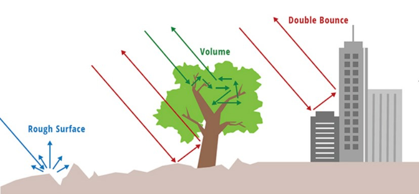
Figure 2 – Types of Radar Backscatter (NASA SAR Handbook)

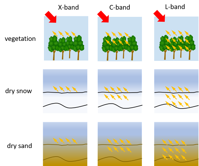
SAR systems operate in different wavelength which has a significant impact on how the radar interacts with the Earth's surface, with longer wavelengths having the ability to penetrate through certain materials such as vegetation, sand, snow, or even dry soil.

• X-band (∼2.5–4 cm) : Very limited penetration, sensitive to small surface features ,commonly used in high-resolution applications (e.g., TerraSAR-X, COSMO-SkyMed).

• C-band (∼4–8 cm) : Medium wavelength, interacts with vegetation canopy and surface structures.

• L-band (∼15–30 cm) : Long wavelength, can penetrates through vegetation and into the soil surface.

  

  Figure 3 : Radar Penetration by Frequency (SAR 101: An Introduction to Synthetic Aperture Radar. Capella Space, 2020)
  

Differences between radar and optical imagery :

1. Spatial resolution and pixel spacing :

In optical imagery, spatial resolution and pixel size are typically the same: the area on the ground represented by one pixel (e.g., 10 m in Sentinel-2). For SAR images, things are a bit more complicated. With SAR, the spatial resolution and pixel spacing (or a pixel's size) are two different things, spatial resolution refers to "the minimum separation between the measurements the instrument is able to discriminate" (NASA SAR Handbook) while pixel spacing refers (like spatial resolution with optical imagery) to the size of the area on the ground represented by one pixel.

SAR images starts with non-square pixels and are later resampled to square pixels.Pixel spacing is always smaller than the actual resolution (ideally pixel spacing should be half the spatial resolution).

2. Acquisition geometry and distortions :

Most spaceborn SAR sensors acquires image with a side-looking geometry. Instead of viewing the surface straight down (as in most optical systems), radar looks at an angle. This results in a radar image being laid out in range (across the look direction) and azimuth (along the flight path).
The side-looking nature of SAR sensors, however, introduces unique geometric distortions that are not present in downward-looking optical imagery.

• Layover : happens with tall objects when the radar beam reach the top of an object before it's base, which in returns means that the top of that object will be placed closer to the sensors on the image, objects will appear collapsed toward the sensor.

• Foreshortening : happens when a slope faces the radar, which leads to distance between the top and base being compressed in the image. Unlike with layover, the order of top and base is preserved.

• Radar Shadow : occurs when a terrain feature blocks the radar signal from reaching an area behind it.

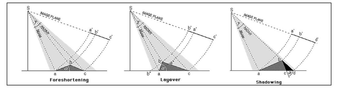
Figure 4 : Distortions present in SAR images (11th Advanced Training Course on Land RS. ESA, 2022)

The direction from which the radar illuminates the scene (ascending or descending) also affects how these distortions appear. Since radar is side-looking, the terrain features will cast layover or shadow in different directions depending on whether the sensor is looking east or west.

To illustrate this last point, we'll take a look at these two SAR images acquired by Capella's Radar 13 and 2 over the Champs-de-Mars in Paris, accessed through Capella's open data gallery. One image (on the left) was acquired during a descending orbit, while the one on the right was taken during an ascending orbit. Both images were captured on a 97° orbital plane by a right-looking satellite.

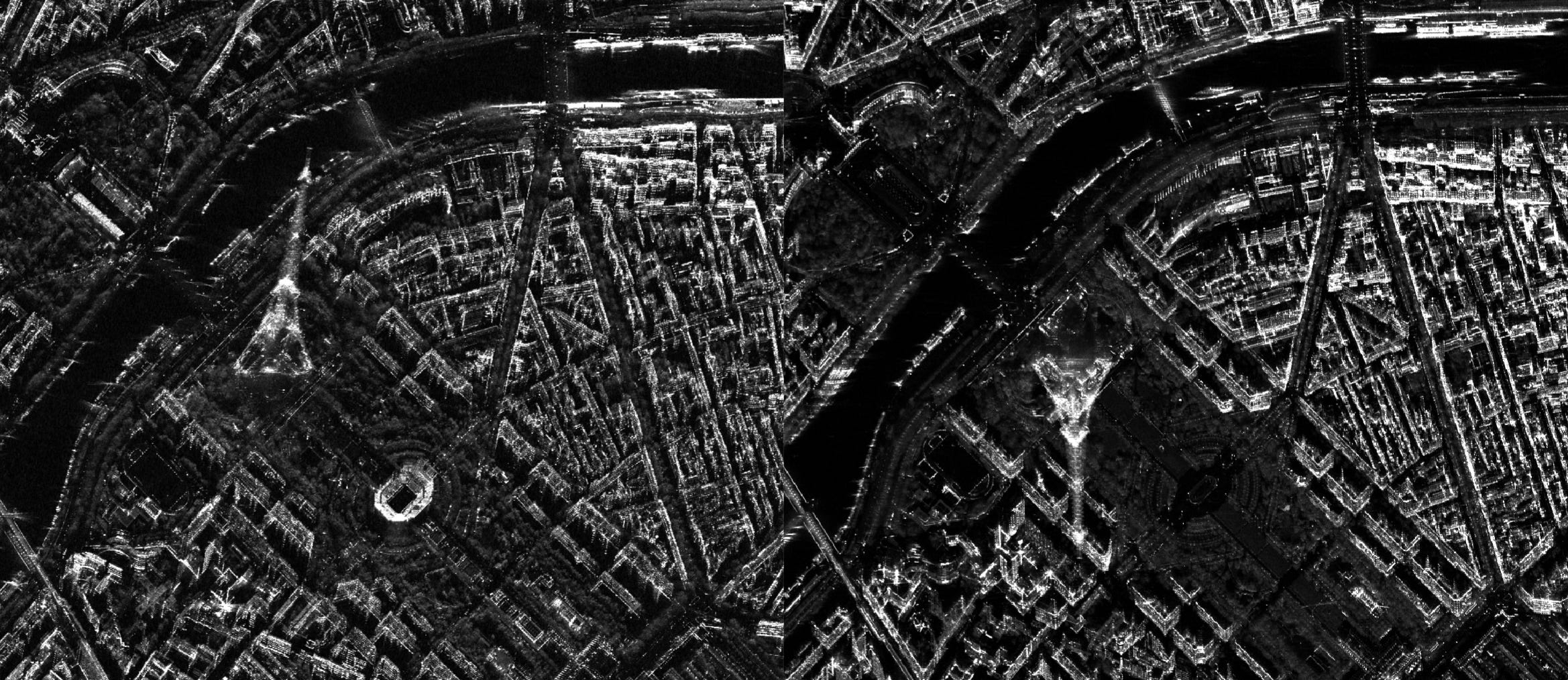
Because of the difference in orbit direction, the viewing geometry changes, and this has a direct effect on how objects are represented in the SAR image. A clear example is the Eiffel Tower, which appears to lean in opposite directions in the two images. The radar "sees" the tower from opposite sides which make it appear laid out toward the radar in the direction of the sensor’s look angle, leading to noticeable layover effects that shift depending on the orbit.

The Sentinel-1 mission :

Sentinel-1 is an ESA mission under the Copernicus Programme, equipped with a C-band SAR sensor for all-weather, day-and-night imaging with a 5 x 20m resolution, and is comprised of three satellites: Sentinel-1A, 1B (inactive since December 2021), and 1C (launched December 2024). Offering freely available data with a typical 6 to 12-day revisit cycle depending on orbit configuration.

S-1 images comes in many different file type/format with the 2 main ones being:

1. Ground Range Detected (GRD) : Contains only intensity (amplitude) information projected onto the ground range, files are lighter and requires less processing (roughly 1gb/image). Ideal for applications such as: land cover classification, flood mapping, surface change detection.

2. Single look complexe (SLC) : contains both amplitude and phase of the signal in radar (slant range) geometry , files are heavier requiring more processing (8gb/image zipped into 4gb). Ideal for applications such as: interferometry (InSAR), coherence change detection (CCD).

Choosing the right Sentinel-1 image :

When choosing the right image to use, it depends entirely on (1) what kind of analysis you're doing which will define what type of file is needed (2) acquisition dates and (3) looking direction.

1. File type : choosing the right image type to use depends entirely on what kind of analysis you're doing. Unless you need the phase information for interferometry or coherence analysis, the recommended product is usually the GRD (Ground Range Detected) format.

2. Dates and number of image : Sometimes when working with SAR images more than one image is required for a reliable analysis. This is due to several factors, such as the presence of speckle noise and the inherent variability in SAR backscatter caused by surface conditions, geometry or atmospheric effects, sometimes requiring an averaging of the backscatter from different acquisition or multi temporal speckle filtering, although speckle might not be an issue when dealing with strong reflector such as urban areas, parked vehicles or for ship detection. This is also relevant with changes detection, as sometimes multiple images might be required in order to establish a baseline or to reliably detect change.

3. Orbit and looking direction : Usually when running any type of change detection algorithme (or any type of algoithme really), it is highly recommended not to mix ascending/descending orbits and stick with the same relative orbit.

   For visual interpretation of SAR images, you can use mix both ascending and descending orbits, as long as you keep in mind that viewing geometry affects how objects appear in order not to interpret the different distortions affecting the image as actual change. Also, depending on orbit direction and incidence angle, the SAR sensor will "see" different sides of a building, mountain, or slope. Which means depending on what you're trying to look at

To illustrate the impact the looking direction can have we'll look at the figure below, It shows the areas identified as "damaged buildings" after running a Coherence change detection algorithm designed just for that, on the left using only images acquired with an ascending orbit and on the right those with a descending orbit. We see that the two building took some damages to the walls facing east.
Using only ascending images we notice that our algorithm was unable to detect these damages. Since sentinel-1 is right looking, with an ascending orbit the radar will image the area from west to east meaning it will face the western side of the building that did not tale any damage with the damaged side invisible to the sensor (radar shadow). With a descending orbit on the other hand, the sensor will face the eastern side of the building which did get damaged and was positively detected as such.

Another interesting detail is how the detected damages appears to be located slightly left of the building, this is due to both layover and the double bounce effect discussed earlier, which lead to the building's footprint on the SAR image being slightly toward the sensor.

Sentinel-1 image processing :

Sentinel-1 SAR images are freely available and can be downloaded from several platforms. I personally use the Alaska Satellite Facility (ASF) Data Search Vertex (https://search.asf.alaska.edu). The Copernicus Browser is also an option, but I find the interface a bit clunky but still great for data visualisation (https://browser.dataspace.copernicus.eu).

While searching for data to download you just need to define an Area of Interest and choose a date range, product type and orbit direction. Once you find an image that suits your needs, I recommend filtering the search results by the relative orbits and frame number that suits you, which should get you all the image in the chosen date range acquired with the same geometry.

The processing of the images will be done using ESA's SNAP and QGIS ideally on a Linux based system (windows is also OK but make sure to make your folder/file names' shorter since you can easily hit windows' "MAX_PATH" limit)

GRD Preprocessing Workflow :

A typical GRD preprocessing workflow would look like shown on figure below in SNAP's Graph Builder

Starting with Radiometric Calibration to sigma nought (σ⁰) (found under RADAR> Radiometric > Calibration) followed by Range Doppler Terrain Correction using a DEM which will be automatically downloaded but you can import your own if your AOI is not covered by SRTM. Optionally, you can also Subset your image and apply Speckle filtering.
If working with multiple images, the final step would "Stack Creation" for image coregistration ensuring pixel alignment across different acquisitions.

Additionally, I like to store all the images into a single .tif file where each bands represent the same scene but on a different day. For this, I use the Virtual Raster tool in QGIS making sure to check the ¨Place each input file into a separate band" box.

SLC Preprocessing Workflow :

Here we'll focus on coherence analysis and Coherence Change Detection (CCD), since InSAR displacement detection in not really useful for GEOINT (maybe for monitoring underground facilities/tunnels and things like that ? I'll make an article about it later on).
A typical SLC preprocessing workflow in SNAP’s Graph Builder looks like show on Fig X. It starts with Orbit correction, TOPSAR split keeping only the bursts we need, followed by back-geocoding (coregistration), coherence estimation and finally terrain correction.

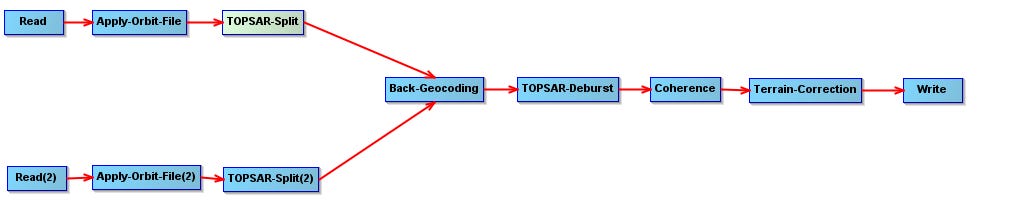
This process results in a coherence map, which highlights stable (high coherence) vs changed or noisy (low coherence) areas between two acquisitions.

Basic histogram manipulation :

As discussed earlier, 16-bit images can be tricky to visualize correctly. SAR images in particular often require histogram stretching or contrast adjustment to be properly visualized.
One important choice when visualizing SAR backscatter is whether to use a linear scale or a logarithmic (dB) scale. While most pixels in a SAR image have relatively low backscatter values, a few pixels (often from urban areas and other strong reflectors) can exhibit very high backscatter (as seen in the histogram example below).
A linear scale will compress lower backscatter values making the image look dim and dark with a only few strong backscatterer visible. Switching to a dB scale will eventually compresses this wide dynamic range and enhances contrast of low backscatter areas. On the image below you can see that when switching from a linear scale (on the left) to a dB scale (on the right) the Max value went from 1180 to 59 which is more manageable.

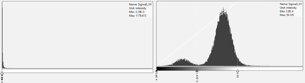
After switching to the dB scale, we notice that we have a trimodal distribution, the lower values are from specular backscatter, followed by a bigger population of pixels from volumetric scatterers and finally pixels from strong reflectors that are less spread out than with a linear scale.

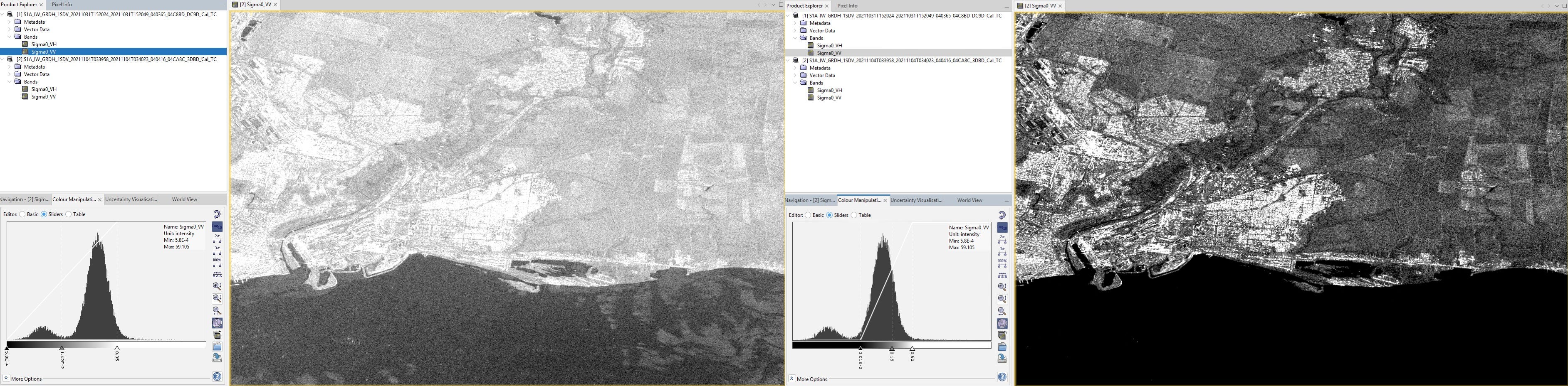
For a better visualisation with the dB scale, I like to put the min slider right after all the specular backscatter then adjust the middle and max sliders until I get balanced image.
When comparing two images it’s necessary to use the same same visualization parameters, one way to do so is to use the “Apply to other bands” function under the color manipulation tab in SNAP, and choosing “No” to the “Automatic distribution between Min/Max.”
On the screenshot below, we see 2 images viewed with different color palette on the left. On the right side we applied the same histogramme stretching for the image above to the one below, we notice now that the city (bright part) no both images now have a similar brightness.

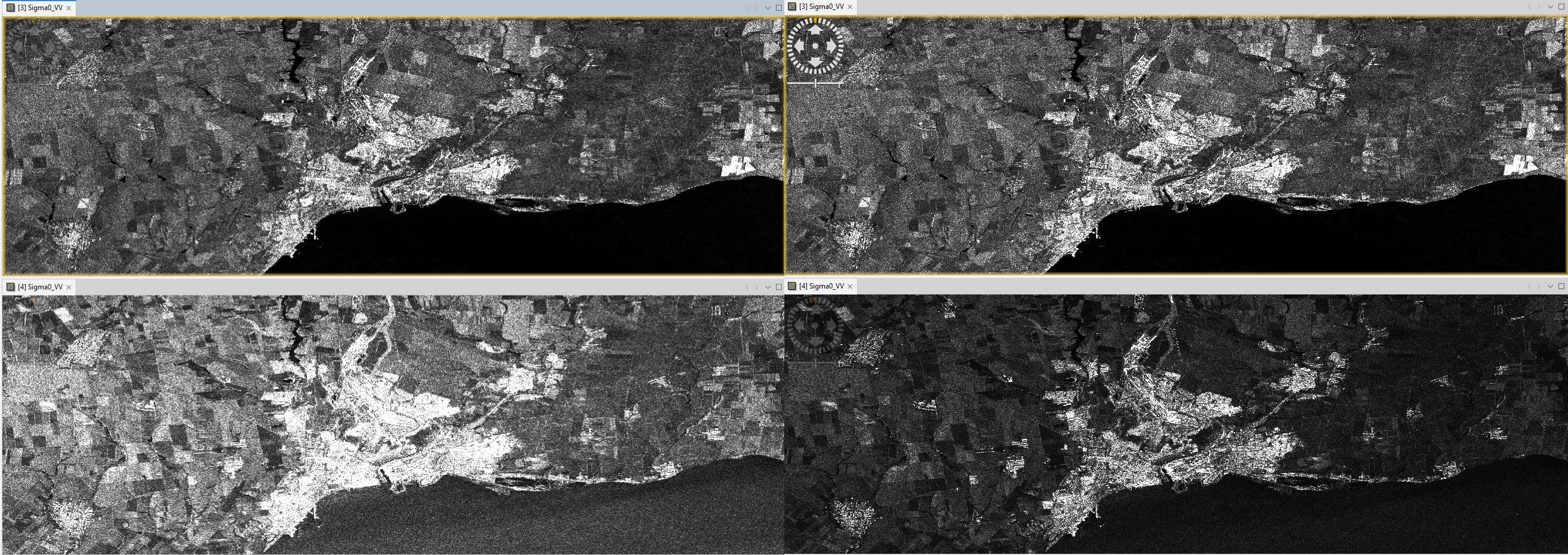
By default SNAP will ignore one part of these high backscatter values as a certain pourcentage of the highest backscatterer which will be attributed the same (highest) shade of grey (more like white). But this is not the case when using QGIS for example, one trick in order to get a more balanced image is to adjust the histogram using the “Local cumulative cut” button on the raster toolbar which should get rid of most of the strong reflector giving you a more balanced image.

Sources :

Capella Space “SAR 101: An Introduction to Synthetic Aperture Radar” : https://www.capellaspace.com/blog/sar-101-an-introduction-to-synthetic-aperture-radar

Capella’s Open Data Gallery : https://www.capellaspace.com/earth-observation/gallery

ESA’s 11th Advanced Training Course on Land RS : https://eo4society.esa.int/training_uploads/LTC2022/1_Monday/9_Introduction2SAR__Ronczyk.pdf

Ogi Gumelar, Liu Dawei , Rahmat Rizkiyanto. Polarimetric Decomposition in Calibrated Radar Image for Detecting Vegetation Object