GEOINT 002 : Monitoring military storage bases with free satellite imagery. Part 1

In this second entry in the GEOINT series, we'll break down how to monitor military activity using freely available optical and SAR satellite imagery.

Jul 21, 2025

On the first of November 2021 Rochan Consulting reported a buildup of ground forces near in Yelnya barracks, based on images Maxar images. Their analysis focused on identifying the units and vehicles deployed there.

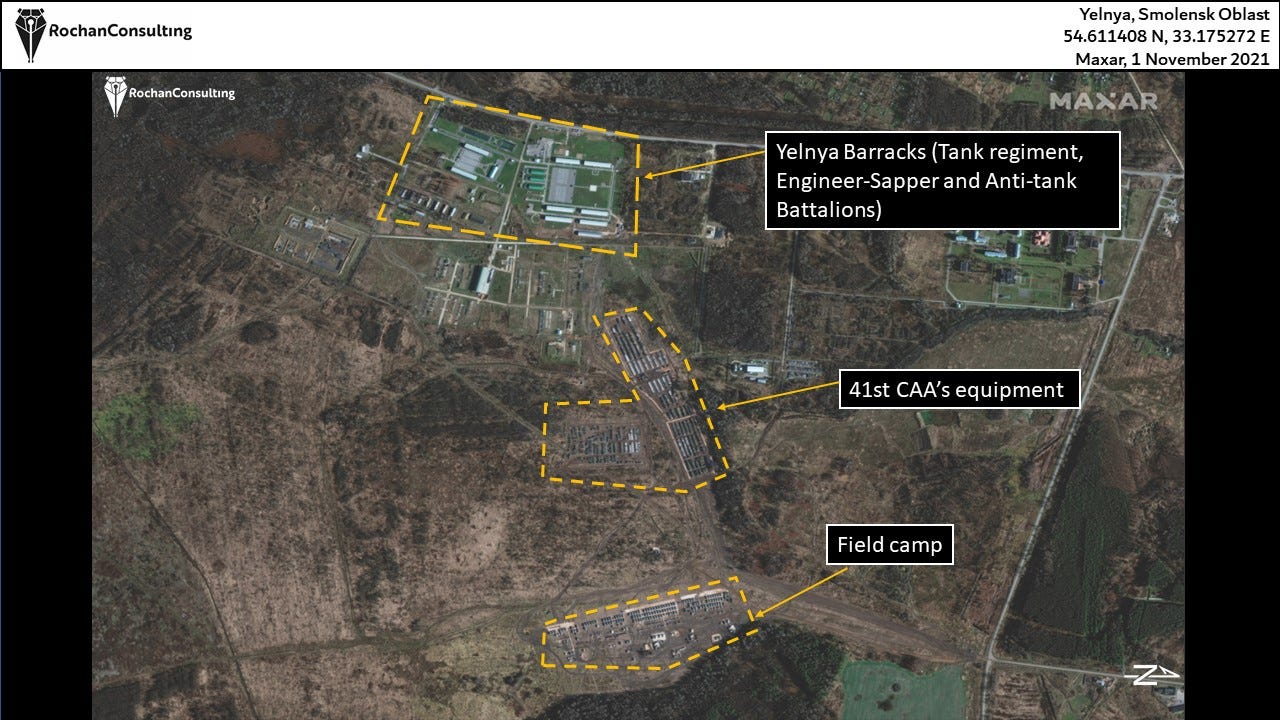
Figure 1 : Expansion of the Yelnya Barracks. (Rochan Consulting. Contains modified Maxar Imagery)

In this article we'll be looking at the same event but with lower resolution optical and radar imagery, the goal is to explore what additional insights we can extract from freely available, medium-resolution satellite data.

The biggest difference when working with medium resolution satellite imagery when compared to the high resolution images (other than being freely accessible) is the frequent revisit time.
When purchasing high-resolution satellite imagery, it's crucial to know the exact date (and sometimes even the time of day) when the event or change you're investigating occurred. This can be particularly be problematic when monitoring a certain area with no clear indication or when "something" might happen, or when working on large areas and not knowing exactly where exactly to look.
This is where medium-resolution, freely available data becomes a good alternative, While lacking in terme of spatial resolution, its frequent coverage and zero cost make it ideal for an initial assessments and to narrow down the timeframe and area of interest.

Before taking a deeper dive into the Yenlya barracks buildup, it's important to first cover the fundamentals of how military storage bases monitoring is typically done using satellite imagery.
Here's a breakdown of the general workflow:

I) Identifying Military Sites of Interest :

The first step is identifying a list of military storage bases, barracks, or airfields to monitor. While this may seem fairly straightforward, it's often far more complex in practice.
For example, on the case study below, the vehicles were parked right outside of perimeter of the barracks. Limiting the monitoring within the fenced perimeter might cause you to miss critical movements or changes, expanding the monitoring area would lead to an increase in resource requirements (storage space, computing power, human intervention for validation…etc).

II) Setting Up a Monitoring Workflow with Medium-Resolution Imagery :

Once sites are identified, the next step is to establish a monitoring workflow using freely available medium resolution imagery.
Medium resolution optical sensors can’t distinguish individual vehicles. Instead, the focus is on classifying the area as either empty or occupied by any vehicles based on image texture. Meaning each pixel would be compared to the neighboring ones, empty parking areas will look smooth with neighboring pixels having similar reflectance. Areas occupied by vehicles would be more textured, meaning the contrast between neighboring pixels will be more pronounced.

Figure 2 : Texture differences between an empty and a vehicle-occupied area with Sentinel-2 Imagery. (Briansk, Russia)

From this classification, I suppose it would technically be possible to estimate the number of vehicles there. If we know their type and how tightly they're packed, we could estimate the area occupied by one vehicle/number of vehicle per unit of area from freely available high resolution imagery (from Google Earth for example) and therefore it possible to get a rough estimate on the number of parked military vehicles from the total area classified as occupied.

With SAR images, things are more complexe (and interesting). On my last post I mentioned that the radar backscatter coefficient (gamma/sigma) is the sum of the backscattered signal over an area, more vehicles means more backscatter and therefore brighter pixels (flat metallic surfaces such as a vehicles's roof are ideal radar reflectors), a sudden increase or decrease of the backscatter over a monitored area indicate a signifiante increase/decrease in the number of vehicles stationed there.

One slight issues we might face while working with SAR data in the presence of strong reflector is the appearance of cross-shaped artifact, this occur when there is only one strong reflector within a pixel which equate to a Dirac distribution, and since the focusing of a synthetic aperture image involve some Fourrier transformations. This will result in 2 well defined "sinc" functions in both range and azimuth. One way to mitigate this is to use the cross-polarized backscatter (VH in the case of Seninel-1 data) which tends to be less affected by these artifacts.

III) High-Resolution Imagery for Detailed Assessment :

Once medium-resolution monitoring detects a significant change, the next step would be acquiring high-resolution imagery (optical or SAR) for a closer look.
With high resolution optical imagery (<1m) it is possible to visually identify and classify individual vehicles, aircraft, or pieces of equipment. This process can even be automatized and scaled up using deep learning–based target recognition models trained on large labeled datasets.

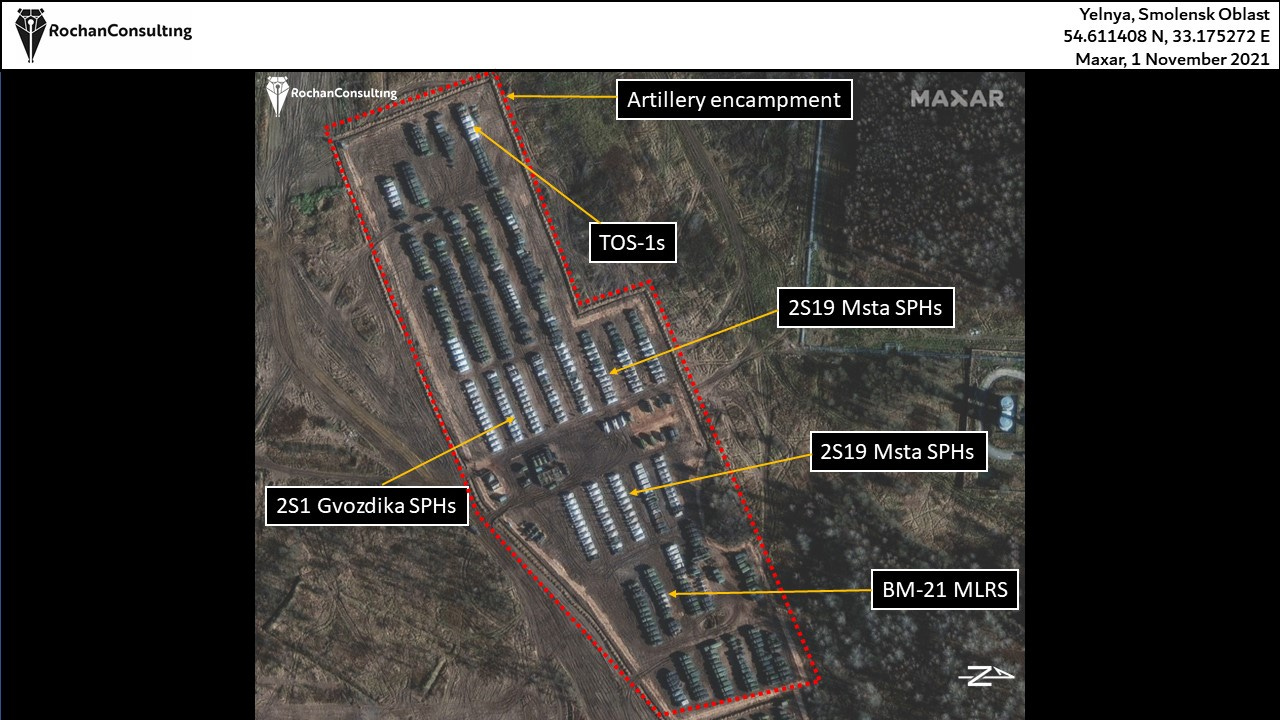
Figure 3 : Military vehicles at at the Yelnya Barracks (Rochan Consulting. Contains modified Maxar Imagery)

However, on a high-resolution SAR image, it's very difficult to tell what type of vehicle you're looking at. This is largely due to the nature of radar imagery, as we can get strong reflections from certain part of the vehicle which can saturate parts of the image, while other parts may produce little or no return (specular reflection). As a result, the object may appear as a bright, blob-like signature with no obvious shape, especially when viewed without context. On the image below we can see one Tupolev Tu-160 and two Tu-22M on a SAR image by Capella (and accessed through Capella’s Open Gallery). Even if we can tell their approximate size and shape, it's difficult to distinguish between the two types

Instead of relying solely on manual interpretation, we typically use Automatic target recognition (ATR) algorithms. As the name suggest, these aim to accurately identify and classify targets of interest in the image such as vehicles, aircraft or ships. These algorithms often relies a variety of techniques most commonly : Deep Learning (CNN), template matching ... etc. And a dataset of images for training purposes, which an either be measured SAR data or simulated.
One of the most commonly used datasets for this task is the "Moving and Stationary Target Acquisition and Recognition (MSTAR)" by the Sandia National Laboratory taken using their X-band SAR sensor, it include a large number of sample image of different military vehicles under different incidence angles.

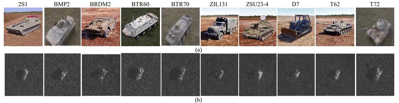
Figure 4 : Examples of standard MSTAR targets (a) visual image (b) SAR image (O. Kechagias-Stamatis, and N. Aouf. 2020)

But still has a few limitations, vehicles appears as small isolated objects with no background clutter which is rarely the case in real life applications, the number of vehicles and scenes it include can also be considered limited by modern standards. Additionally due to the multitude of parameters that affects SAR images and complexe nature of the scattering mechanisms, this datasets might not always be suitable.

Which leads us o the next type of data that can be used : Simulated SAR data.
SAR simulation algorithm can reproduce the working process of SAR systems and generate images of a target as seen by different SAR sensors under different viewing conditions and with complexe backgrounds.

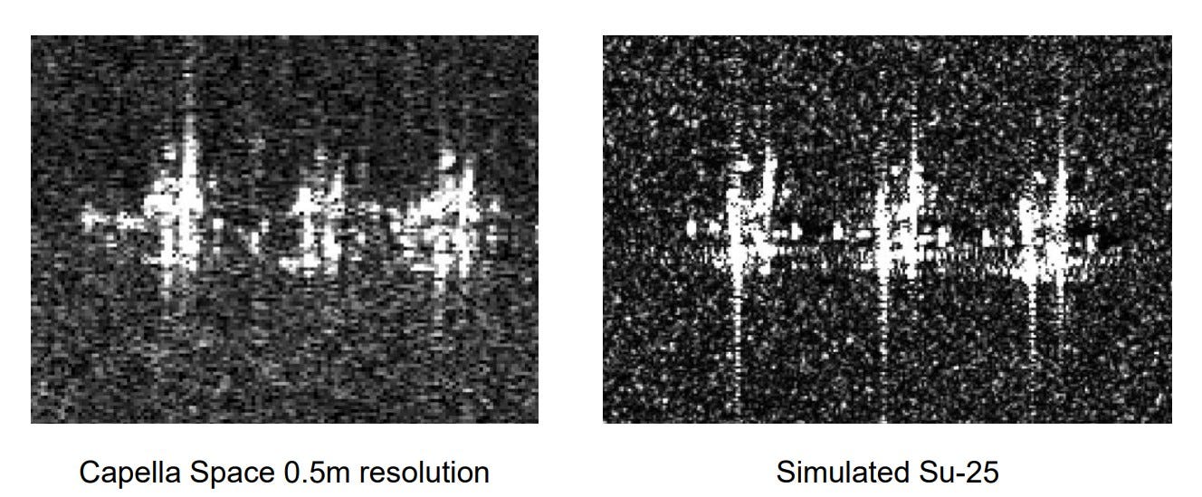
Figure 5 : 3 Su-25 on a Capella space Image next to 3 simulated Su-25 (SARMAP SA/ NV5 Geospatial. 2020)

On the image above we can see 3 Su-25 on an image by Capella space, next to them a simulated SAR image with the same targets. We can see that the simulated image gets pretty close to the measured one. The simulations requires an accurate 3D models of the target, definitions of material properties, sensors parameters (incidence angle, azimuth, wavelength, polarization…Etc).

Case study N1 : The Yelnya Barracks.

Now we'll take a look at the same event using freely available satellite imagery and see what additional insight we can extract from them.
We will try to answer a few basic question : When did the vehicles get there ? An how long did hey stay there ?.

Sentinel-2 image were accessed through the Copernicus Browser without any local processing. With Sentinel-2 we notice that already on the 29/09, there were signs of troop movements, no vehicles build-up yet but on a false color composite with the NIR band, we can see traces of repeated vehicle passage and early terrain preparation. During the month of October there was a gradual increase in the number of parked vehicles, but due to cloud cover very few images are usable around this time of the year, with a peak in the number of vehicles reached on the first of November.

The next cloud-free images was taken next January 2022, where we can still see vehicles present at the site. One interesting thing on this image is that, due to snow cover, we can clearly see the differences in texture between areas with and without vehicles. And finally we get another cloud free image on the 24th of February, even if the image is difficult to interpret we can tell that the vehicles have already left the area. Since the area where they used to be are not completely covered in snow like the surrounding fields.

This again highlight the main advantage of working with SAR imagery, as it offers imaging capabilities under all weather conditions, which can be essential particularly for some time sensitive applications such as this one.

Switching now to Sentinel-1 SAR images we'll follow the same workflow mentioned in the previous post. I have also included a step by step guide with screenshot toward the end of this post. We’ll be processing the 22 GRD images taken between 09/2021 and 03/2022.
Our analysis will be done in QGIS, using the “Temporal/Spectral Profile Tool” plugin to view the backscatter time series, we'll also be using multi temporale color composites to view changes between different dates. As a basemap we’ll be using ESRI’s satellite basemap accessed via the “QuickMapServices” plugin and which is composed of the same Hires imagery from Maxar as the article mentioned earlier and which we used to validate out findings.

One of the simplest way to visualize change between two images, is to make false color composite using images acquired on 2 different dates. Here, we'll view band 8 on our image (image acquired on the 31 of October) with the Blue and Green color, and with Red we'll view the first band (and first image) of our stack.
Places with strong backscatter on both the image we'll be visible in white, strong backscatter on the 2nd date (during the peak of buildup) that wasn't present on the first image we'll be visible in cyan. Inversely strong backscatter only on the first date will be present in Red.

Red : Ɣ⁰ 19/09/2021 Green : Ɣ⁰ 31/10/2021. Blue : Ɣ⁰ 31/10/2021

We can already see the areas where the vehicles were parked visible in cyan on the images above(ie areas with strong backscatter on the 31/10 image only) this means we had an increase in backscatter on the chosen date (31/10). But we notice on the western side (2nd image) the tents installed there didn’t not cause any strong backscatter, as the materials and their general shape are not ideal radar reflectors.

Now that we identified the areas occupied by vehicles, the next step we'll be to visualize the backscatter time series, in order to track changes in activity over time.

We notice an increase starting from band 8 (acquired on the 31/10) gamma⁰ values then stays relatively high for most of the TS then drops suddenly in some areas starting from band 20 (04/02/2022) and in other from band 21 (16/02/2022).

When viewing time series it is important to examine multiple locations within the region of interest (ROI) as SAR backscatter values can have random values sometimes. Only after observing the same pattern across several neighboring pixels, does it become safe to interpret it as a real change or event.

It is also necessary to visually inspect the imagery for multiple dates in addition to analyzing the time series, to make sure we don’t miss any critical details.
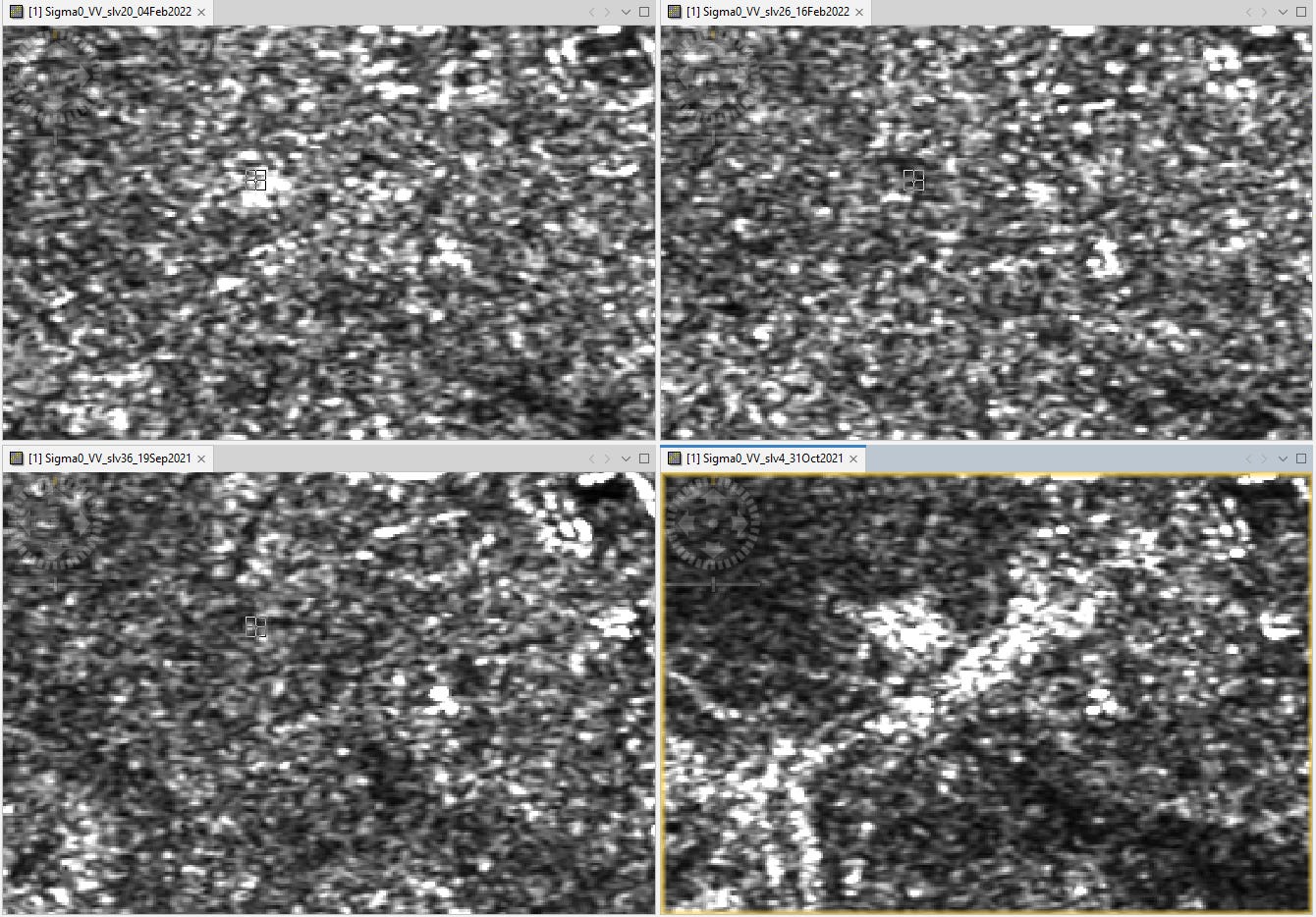
On the image below we can see out ROI at different times. On the bottom left the image was taken on the 19/09 before any vehicle showed up, on the right it was taken on 31/10 we can see bright pixels where the vehicles were parked. The top two images were taken on the 04/02 (band 20) and 16/02 (band 21), on the first one we can see that we still have some bright pixels in our ROI, but on the 16th of February the vehicles were all gone. Which indicate that moved out gradually during that time.

Conclusion :

This case study shows that with the right tools and methods freely available medium resolution optical and radar satellite imagery offers a practical way to monitor ground targets, especially when frequent coverage over wide areas is needed even when lacking the spatial detail of commercial high-resolution imagery.

Sources :

SARMAP/NV5 Geospatial : SAR Image Simulation and Automatic Target Recognition https://www.nv5geospatialsoftware.com/Portals/0/pdfs/SAS/3_Paolo_Pasquali.pdf

O. Kechagias-Stamatis, and N. Aouf. Automatic Target Recognition on Synthetic Aperture Radar Imagery: A Survey. https://arxiv.org/pdf/2007.02106

Capella’s Open Data Gallery : https://www.capellaspace.com/earth-observation/gallery

Rochan Consulting. Yelnya Barracks – Analysing Maxar’s image : https://rochan-consulting.com/yelnya-barracks-analysing-maxars-image/